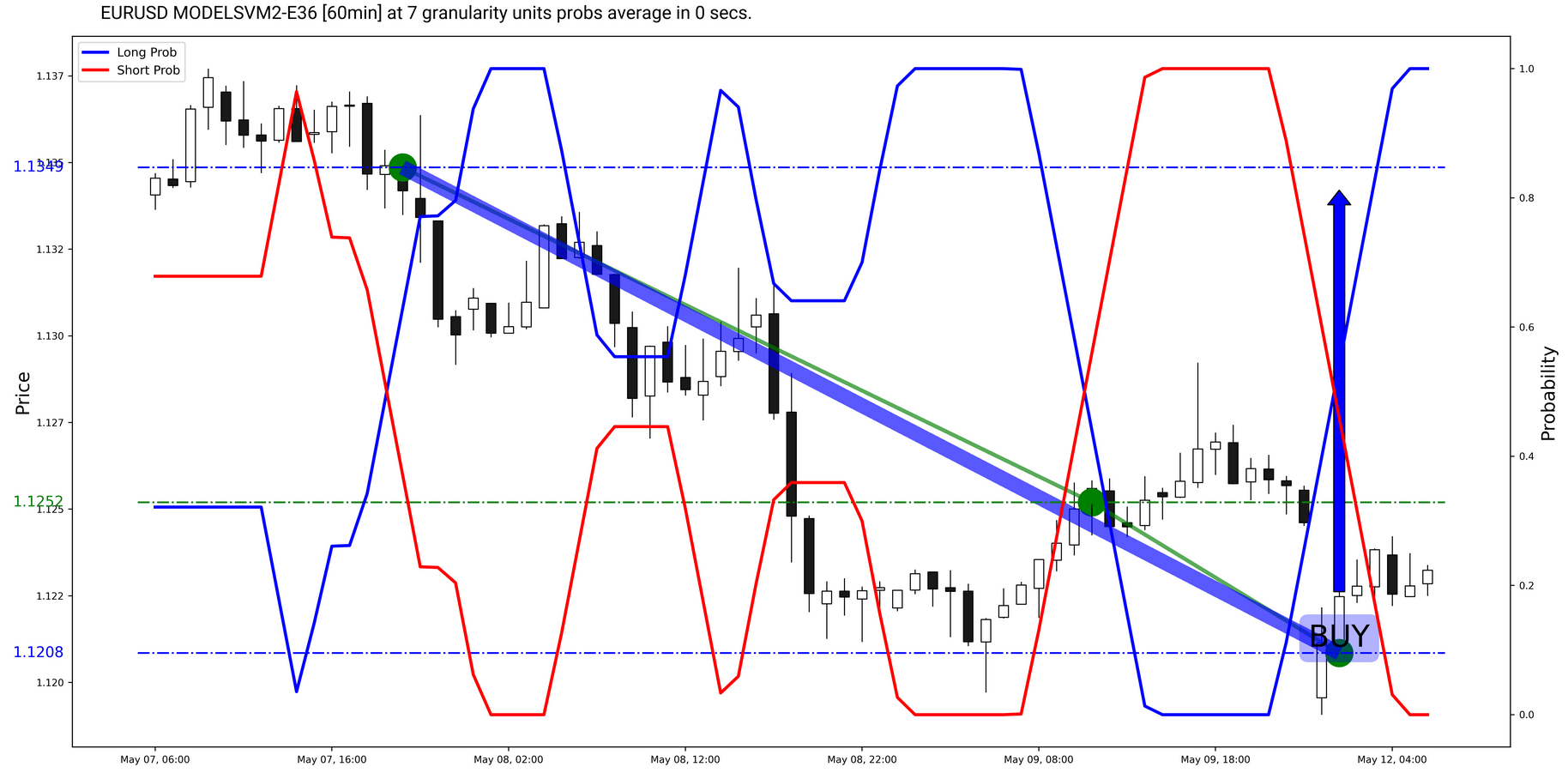
The EURUSD has done a false down move from 1.1349 to 1.1252. When the market opened today, the probability trend reversed back to long, so now now we expect an upward reversal from 1.1208 to 1.1349.
Figure 1 EURUSD Outlook

1. Background
Our models generate estimates about the price movements of financial instruments. They calculate the probabilities for an up or down movement of the spot price in a predefined during training look-ahead period. They do that at short time intervals. The results are then averaged, according to user preferences, until the chart loses the noise and gains focus.
Different models may have been trained on data, containing different features structure. We have also used different model types, including support vector machines (SVMs), gradient boost (xgboost) models or hybrid convolutional/lstm models.
2. Definitions - the Period Structure
The models split the price movement into consecutive periods of long and short probability trends. We can define these fragments as time intervals in which the respective probability is dominating. These periods are on the chart, no matter what model, instrument, granularity level or probability averaging parameter we chose. Of, course, changing the above settings alters the outlook of these periods. Trend periods have several describing characteristics.
• They could be either long or short, depending on the dominant probability.
• They have a start time/price (bid) level.
• They have a prob-max point, with a probability value and a time / price (bid) level.*
• They have an end time/price (bid) level.
*For the SVMs, which generate only 0 and 1 probabilities, the prob-max value is a pretty relative average.
We refer to the line, which connects the trend-change points as the trend-line.
We can visualize our definitions on the chart in Figure 1
.
Figure 1 Periods on the Chart

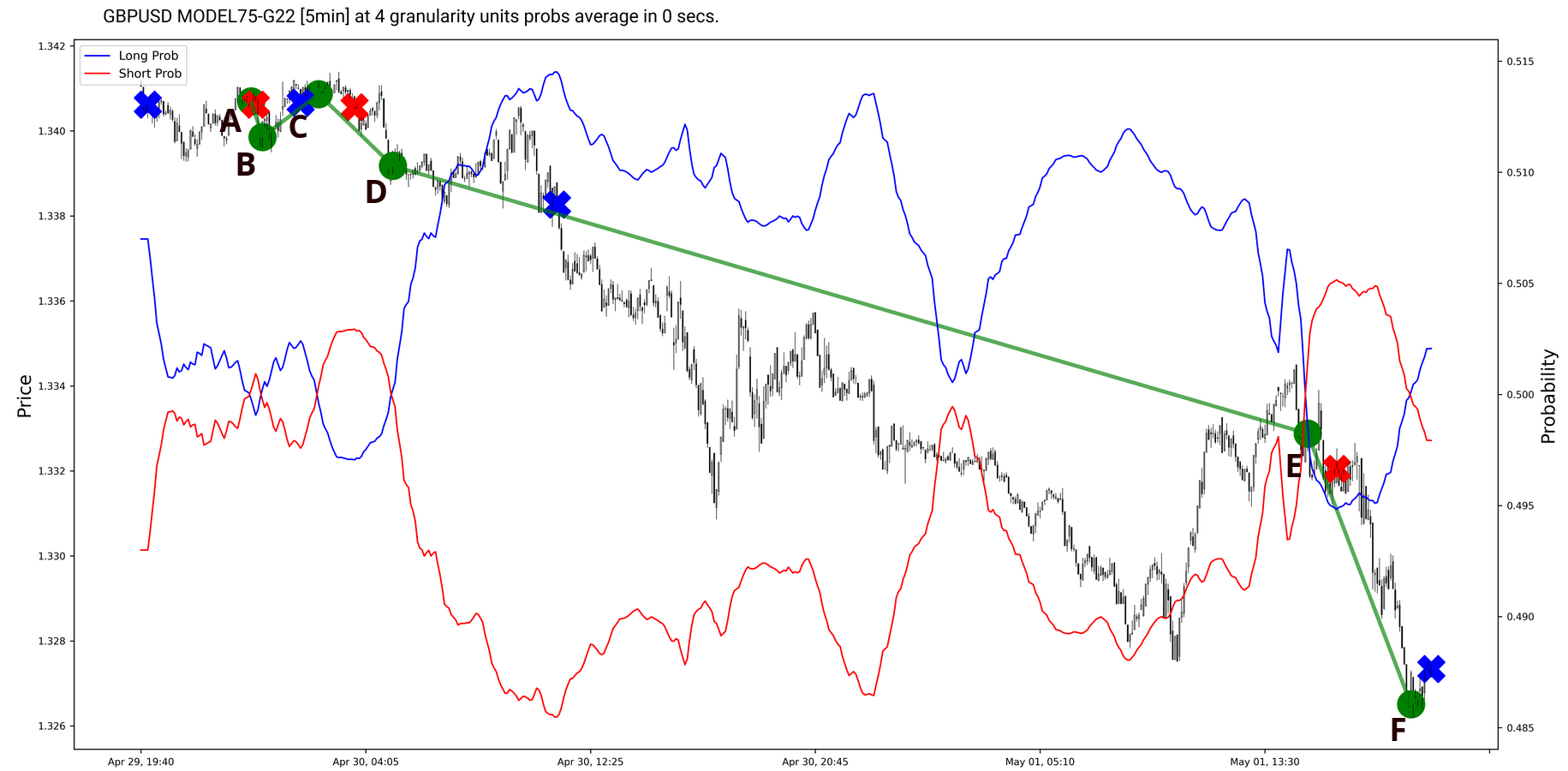On this figure we have five periods, namely AB, BC, CD, DE and EF, determined by the probability trend change points, colored in green. Each of these period has a dominant probability, which determines the sign of the period - AB is a short period, BC is long, CD is short, DE is long and EF is short. They also have a prob-max point, depicted by the X sign of the respective color. The price/time coordinates of the green trend-change points mark the beginning and the end of the periods. The green line, connecting the dots, is our trend-line.
3. Simplifications
We say that if the trend-line of a short period has a downward slope and if the trend-line of a long period has an upward slope - the model has performed well. On the flip side, if the reverse holds true - the model has done poorly and we have a false prediction or an exception. So, on the chart in Figure 1, the model has done well predicting the movement in the periods AB, BC, CD and EF. The model has performed poorly in period DE. We will make this assumption, regardless of whether we have a probabilistic or a non-probabilistic model.
Conventionally, for the soft (probabilistic) classifiers, in order to assess the model visually, we look at the prob-max points. In this context the price movement should be explained by the consecutive long and short probability maxima. From a trader’s point of view, we should buy the long probability maxima and sell the short probability maxima. In order to illustrate our point, however, we will simplify and say that the prediction is either true or false, based on period’s trend-line and probability sign and that deviations from the period’s trend-line are simply volatility.
4. Trading the Exceptions Moves
So, we have divided the price movements of the trading instruments in long and short periods, according to the model’s assessment and we have stipulated that the model’s predictions for such periods could be either true or false.
Price, however, makes up for the model’s false predictions and the compensating move usually starts in the next period of the same sign. We can illustrate our point in Figure 2, which is the same trading instrument in somewhat longer time span.

Figure 2 Coverage of an Exception Period

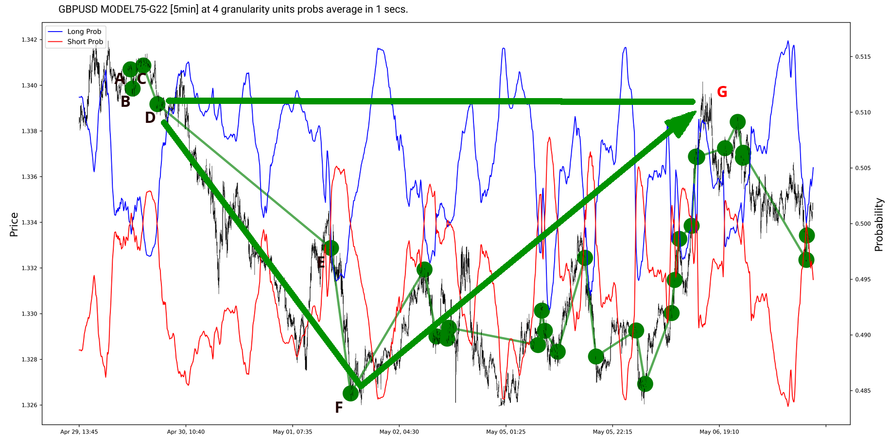As noted in Figure 1, in Figure 2 we have a falsely predicted period, which is DE. There the model expects an up move, but the price is actually going down. Price covers for the mistake, which the model has made, with a move starting in next long period, which is the long period starting at point F. After a rather complicated and long winding, the price lands at point G, which is not on the trendline, and covers for the DE move. In doing so, it predicts a false down move and will cover this second false prediction, but that is outside the scope of our illustration, because it repeats the same principle.
We are of the opinion, that this concept explains a large portion of the big price movements and can be used to traders’ advantage. Here we have not only the starting point, but also the take-profit level, which is the point, covering the initially incorrect prediction.
5. Areas of Improvement
The statement we are making is backed by experience only. We cannot prove it mathematically. What is more, we do not actually know why is this happening. Of course, we may think that, at some point, there is some noise going into the system and the system is trying to compensate for its temporary reaction to that noise. If this is the case, if such events come close and corrections overlap, what is the sequence in which the system restores its equilibrium? We are also not sure what these events are or are they actually events or market sentiments for future events. Probably, when the market makes a sufficiently big move in a direction contrary to probability, fundamentals tend to reverse the move. At any rate, this should have been caught during training.
Also, we can not say the exact granularity and probability averaging parameters, at which this phenomenon becomes visible. We assume that these may change in response to market intensity or the quantities traded. The settings will be different for the different models at different times. Currently, clients have to work with the charts and the models, in order to find out which outlook fits best and identify the trades.

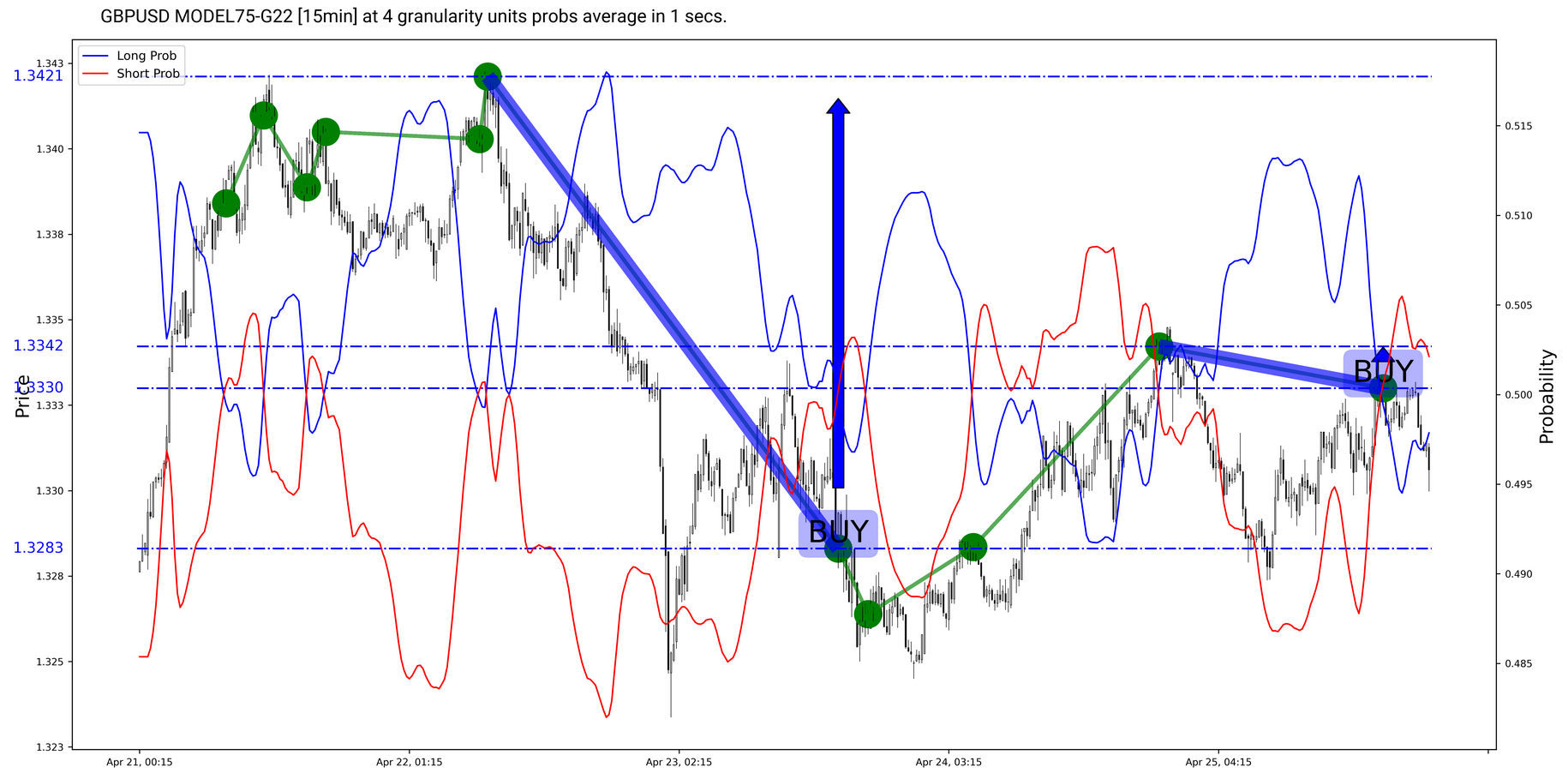We can see that the GBPUSD has taken a nosedive on a long probability trend from 1.3421 to 1.3283. We think that the market will make a compensatory move back up. In the meantime, the market has moved up on a short probability trend from 1.3283 to 1.3342, but has covered for the move immediately after.

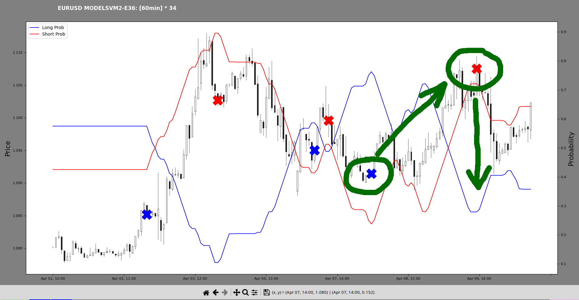Based on the current context, we expect a downward move in towards the 1.0915 level, where we had a previous up probability high.

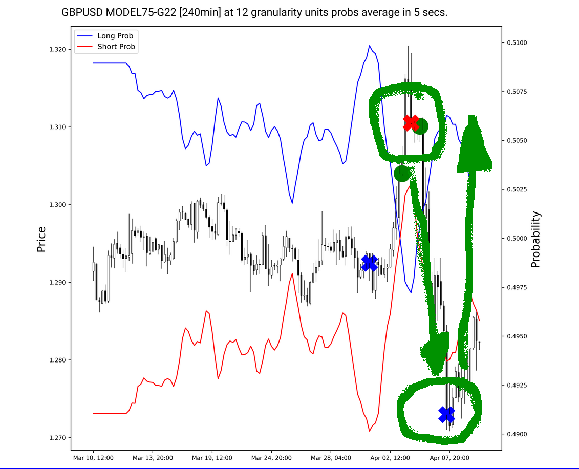The upward probability has spiked at 1.2730, so we expect an upward move. Although the downward probability has not yet topped, an intermediary target could be the previous high at 1.3105.